Conduct Randomization Inference — conduct

This function makes it easy to conduct three kinds of randomization inference.

Usage

conduct_ri(
  formula = NULL,
  model_1 = NULL,
  model_2 = NULL,
  test_function = NULL,
  assignment = "Z",
  outcome = NULL,
  declaration = NULL,
  sharp_hypothesis = 0,
  potential_outcomes = NULL,
  studentize = FALSE,
  IPW = TRUE,
  sampling_weights = NULL,
  clusters = NULL,
  permutation_matrix = NULL,
  data,
  sims = 1000,
  progress_bar = FALSE,
  p = "two-tailed"
)

Arguments

formula: an object of class formula, as in lm. Use formula when conducting significance tests of an Average Treatment Effect estimate under a sharp null hypothesis. For the difference-in-means estimate, do not include covariates. For the OLS covariate-adjusted estimate, include covariates. Transformations of the outcome variable such as log(Y) ~ Z are supported.
model_1: an object of class formula, as in lm. Models 1 and 2 must be "nested." model_1 should be the "restricted" model and model_2 should be the "unrestricted" model.
model_2: an object of class formula, as in lm. Models 1 and 2 must be "nested." model_1 should be the "restricted" model and model_2 should be the "unrestricted" model.
test_function: A function that takes data and returns a scalar test statistic.
assignment: a character string that indicates which variable is randomly assigned. Defaults to "Z".
outcome: a character string that indicates which variable is the outcome variable. Defaults to NULL.
declaration: A random assignment declaration, created by declare_ra.
sharp_hypothesis: either a numeric scalar or a numeric vector of length k - 1, where k is the number of treatment conditions. In a two-arm trial, this number is the hypothesized difference between the treated and untreated potential outcomes for each unit. In a multi-arm trial, each number in the vector is the hypothesized difference in potential outcomes between the baseline condition and each successive treatment condition.
potential_outcomes: an optional character vector naming one column of data per treatment condition, giving each unit's hypothesized outcome under that condition. Columns are matched to conditions in sorted order. Supplying this states the sharp hypothesis directly and allows hypothesized effects that vary across units, which sharp_hypothesis cannot express. Each unit's observed outcome must be preserved in the column matching the condition it was actually assigned to; only the other columns are hypothesized counterfactuals. Cannot be combined with a non-zero sharp_hypothesis.
studentize: logical, defaults to FALSE. Should the test statistic be the t-ratio rather than the estimated ATE? T-ratios will be calculated using HC2 robust standard errors, or CR2 clustered standard errors when clusters is specified.
IPW: logical, defaults to TRUE. Should inverse probability weights be calculated?
sampling_weights: a character string indicating which variable in data contains sampling weights. Sampling weights are fixed across permutations (they reflect the sampling design, not the assignment). When combined with IPW = TRUE, sampling and inverse probability weights are multiplied together.
clusters: a character string indicating which variable in data contains the cluster IDs. When supplied with studentize = TRUE, CR2 clustered standard errors are used instead of HC2.
permutation_matrix: An optional matrix of random assignments, typically created by obtain_permutation_matrix.
data: A data.frame.
sims: the number of simulations. Defaults to 1000.
progress_bar: logical, defaults to FALSE. Should a progress bar be displayed in the console?
p: Should "two-tailed", "upper", or "lower" p-values be reported? Defaults to "two-tailed". For two-tailed p-values, whether or not a simulated value is as large or larger than the observed value is determined with respect to the distance to the sharp null.

Details

1. Conduct hypothesis tests under the sharp null when the test statistic is the difference-in-means or covariate-adjusted average treatment effect estimate. 2. Conduct "ANOVA" style hypothesis tests, where the f-statistic from two nested models is the test statistic. This procedure is especially helpful when testing interaction terms under null of constant effects. 3. Arbitrary (scalar) test statistics

Examples


# Data from Gerber and Green Table 2.2

table_2.2 <-
    data.frame(d = c(1, 0, 0, 0, 0, 0, 1),
               y = c(15, 15, 20, 20, 10, 15, 30))

## Declare randomization procedure
declaration <- randomizr::declare_ra(N = 7, m = 2)

## Conduct Randomization Inference
out <- conduct_ri(y ~ d,
                  declaration = declaration,
                  assignment = "d",
                  sharp_hypothesis = 0,
                  data = table_2.2)

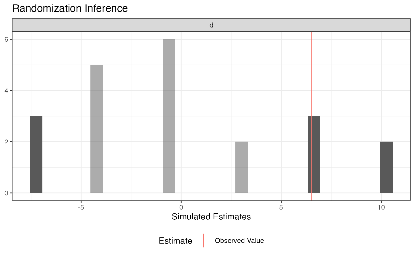
summary(out)
#>   term estimate two_tailed_p_value
#> 1    d      6.5          0.3809524
plot(out)

tidy(out)
#>   term estimate   p.value
#> 1    d      6.5 0.3809524

# Using a custom permutation matrix

permutation_matrix <-
 matrix(c(0, 0, 0, 0, 0, 0, 1,
          0, 0, 0, 0, 0, 1, 0,
          0, 0, 0, 0, 1, 0, 0,
          0, 0, 0, 1, 0, 0, 0,
          0, 0, 1, 0, 0, 0, 0,
          0, 1, 0, 0, 0, 0, 0,
          1, 0, 0, 0, 0, 0, 0),
        ncol = 7)

conduct_ri(y ~ d, assignment = "d", data = table_2.2,
           permutation_matrix = permutation_matrix)
#>   term estimate two_tailed_p_value
#> 1    d      6.5          0.2857143


# Randomization Inference for an Interaction

N <- 100
declaration <- randomizr::declare_ra(N = N, m = 50)

Z <- randomizr::conduct_ra(declaration)
X <- rnorm(N)
Y <- .9 * X + .2 * Z + 1 * X * Z + rnorm(N)
dat <- data.frame(Y, X, Z)

ate_obs <- coef(lm(Y ~ Z, data = dat))[[2]]

out <-
  conduct_ri(
    model_1 = Y ~ Z + X,
    model_2 = Y ~ Z + X + Z * X,
    declaration = declaration,
    assignment = "Z",
    sharp_hypothesis = ate_obs,
    data = dat, sims = 100
  )

plot(out)

summary(out)
#>          term estimate two_tailed_p_value
#> 1 F-statistic 15.22457                  0

# Randomization Inference for arbitrary test statistics

N <- 100
declaration <- randomizr::declare_ra(N = N, m = 50)

Z <- randomizr::conduct_ra(declaration)
X <- rnorm(N)
Y <- .9 * X + .2 * Z + rnorm(N)
dat <- data.frame(Y, X, Z)

balance_fun <- function(data) {
    f_stat <- summary(lm(Z ~ X, data = data))$f[1]
    names(f_stat) <- NULL
    return(f_stat)
}

out <-
  conduct_ri(
    test_function = balance_fun,
    declaration = declaration,
    assignment = "Z",
    sharp_hypothesis = 0,
    data = dat, sims = 100
  )

plot(out)

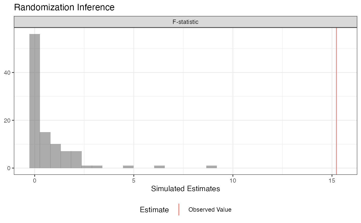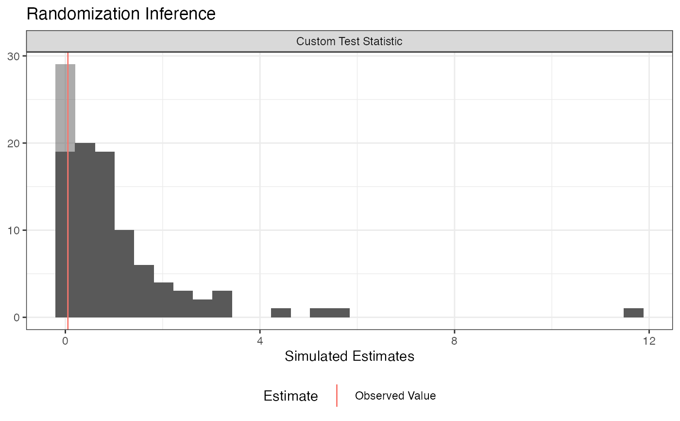summary(out)
#>                    term   estimate two_tailed_p_value
#> 1 Custom Test Statistic 0.05245928                0.9
tidy(out)
#>                    term   estimate p.value
#> 1 Custom Test Statistic 0.05245928     0.9