Drawing the extreme value bounds

estimator_ev() reports a range of average treatment effects rather than a point, and the range comes from filling in the missing outcomes twice: once with the worst case for the treatment group, once with the best. That imputation can be drawn, and drawing it is the fastest way to see what the estimator is doing. This vignette puts the picture and the estimates side by side and checks that they are the same thing.

The plot uses vayr and the difference in means uses estimatr. Both are suggested packages rather than required ones, so if either is missing the code below is shown but not run. impute_extreme_values() and the attrition_experiment data arrived in vayr 1.1.0, so the same is true against an earlier version. The requirement lives in the chunk guard rather than in Suggests, because a version constraint there cannot be satisfied from CRAN until 1.1.0 is released.

library(attrition)
library(vayr)
library(estimatr)
library(ggplot2)
library(dplyr)
#> 
#> Attaching package: 'dplyr'
#> The following objects are masked from 'package:stats':
#> 
#>     filter, lag
#> The following objects are masked from 'package:base':
#> 
#>     intersect, setdiff, setequal, union

The experiment

vayr::attrition_experiment is a simulated two-arm trial with 200 subjects and a seven-point Likert outcome. Nineteen subjects have no outcome, and their missingness is related to the outcomes they would have reported, so dropping them conditions the analysis on a post-treatment variable.

dat <- attrition_experiment

dat |> count(Z, R)
#> # A tibble: 4 × 3
#>       Z     R     n
#>   <dbl> <dbl> <int>
#> 1     0     0    10
#> 2     0     1    90
#> 3     1     0     9
#> 4     1     1    91

The picture

vayr::impute_extreme_values() does the imputation and nothing else. It returns both scenarios stacked, with a flag marking which points were reported and which were filled in.

bounded <- impute_extreme_values(dat, outcome = "Y", assignment = "Z", range = c(1, 7)) |>
  mutate(condition = if_else(Z == 1, "Treatment", "Control"))

bound_means <- bounded |>
  group_by(condition, scenario) |>
  reframe(tidy(lm_robust(Y ~ 1))) |>
  mutate(Y = estimate)

The nineteen orange points are the imputations. In the left panel they sit at the bottom of the scale for treated subjects and at the top for control subjects, which is the least favorable arrangement the data admit. The right panel reverses them. The black points are the arm means either way.

gg_df <- bounded

# Labelled in the left panel only. The colours carry over to the right one, and
# a second copy of the same two words would just be more ink.
label_df <- gg_df |>
  distinct(scenario, imputed) |>
  filter(scenario == "Lower bound") |>
  mutate(
    condition = "Control",
    Y = if_else(imputed == "Outcome imputed", 7, 5),
    label = if_else(imputed == "Outcome imputed", "imputed", "reported")
  )

ggplot(gg_df, aes(condition, Y)) +
  geom_point(aes(colour = imputed, shape = imputed),
             position = position_sunflower(density = 45, aspect_ratio = 0.45),
             alpha = 0.5, stroke = 0) +
  geom_point(data = bound_means, size = 3) +
  geom_errorbar(data = bound_means, aes(ymin = conf.low, ymax = conf.high), width = 0) +
  geom_text(data = label_df, aes(label = label, colour = imputed),
            hjust = 0, nudge_x = 0.2, size = 3.2, show.legend = FALSE) +
  facet_wrap(~ scenario) +
  scale_colour_manual(values = c("#205C8A", "#C67800")) +
  scale_y_continuous(breaks = 1:7) +
  labs(x = NULL, y = "Outcome [1: strongly disagree, 7: strongly agree]") +
  theme(legend.position = "none")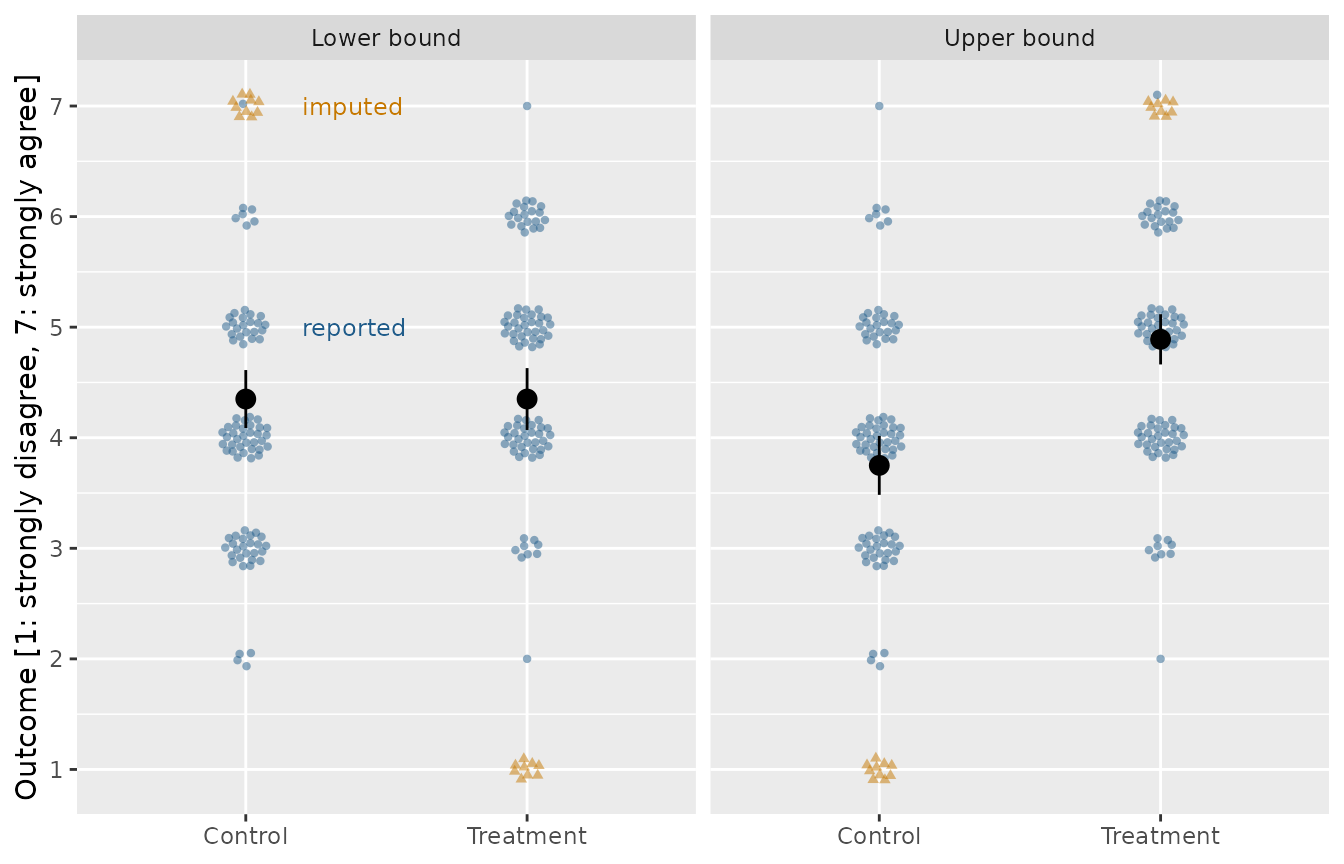

The estimates

estimator_ev() takes the same substantive input, the logical minimum and maximum of the outcome, and returns the two bounds with a joint confidence interval.

ev <- estimator_ev(Y, Z, R, minY = 1, maxY = 7, data = dat)
ev
#>   ci_lower   ci_upper    low_est    upp_est    low_var    upp_var 
#> -3.170e-01  1.430e+00  8.882e-16  1.140e+00  3.715e-02  3.106e-02

tidy() puts the same object in a data frame, one row for the interval and one for each bound, which is the form the comparison below wants.

tidy(ev)
#> # A tibble: 3 × 8
#>   term         estimate std.error conf.low conf.high estimate.low estimate.high
#>   <chr>           <dbl>     <dbl>    <dbl>     <dbl>        <dbl>         <dbl>
#> 1 bounds      NA           NA       -0.317      1.43     8.88e-16          1.14
#> 2 lower_bound  8.88e-16     0.193   NA         NA       NA                NA   
#> 3 upper_bound  1.14e+ 0     0.176   NA         NA       NA                NA   
#> # ℹ 1 more variable: outcome <chr>

The bounds are the two pictures. A difference in means run inside each panel recovers the two bound estimates to the twelfth decimal place, because filling in the missing outcomes and averaging is all the estimator does to reach its point estimates. They are the same calculation reached from two directions.

by_scenario <- bounded |>
  group_by(scenario) |>
  reframe(tidy(lm_robust(Y ~ Z))) |>
  filter(term == "Z") |>
  mutate(term = if_else(scenario == "Lower bound", "lower_bound", "upper_bound")) |>
  select(scenario, term, difference_in_means = estimate, conf.low, conf.high)

by_scenario |>
  left_join(tidy(ev) |> select(term, estimator_ev = estimate), by = "term") |>
  select(scenario, difference_in_means, estimator_ev) |>
  mutate(across(c(difference_in_means, estimator_ev), \(x) round(x, 12)))
#> # A tibble: 2 × 3
#>   scenario    difference_in_means estimator_ev
#>   <fct>                     <dbl>        <dbl>
#> 1 Lower bound                0            0   
#> 2 Upper bound                1.14         1.14

What the picture cannot show

The error bars in the plot are ordinary confidence intervals around four arm means, one panel at a time. They do not answer the question the estimator answers, which is how far the identification region has to be widened to cover the true effect at the stated confidence level.

The tempting move is to take the outermost endpoints of the two panels and call that the interval. It is wider than necessary. The Imbens-Manski interval covers the parameter with probability 0.95 rather than covering the whole identified set, and it uses the fact that the true effect cannot sit at both ends at once.

bind_rows(
  by_scenario |>
    summarise(interval = "Stacking the two panels",
              lower = min(conf.low),
              upper = max(conf.high)),
  tidy(ev) |>
    filter(term == "bounds") |>
    transmute(interval = "Imbens-Manski", lower = conf.low, upper = conf.high)
) |>
  mutate(width = upper - lower)
#> # A tibble: 2 × 4
#>   interval                 lower upper width
#>   <chr>                    <dbl> <dbl> <dbl>
#> 1 Stacking the two panels -0.381  1.49  1.87
#> 2 Imbens-Manski           -0.317  1.43  1.75

Saying the range out loud

minY and maxY here are the same two numbers as range there, and neither function will guess them. That is deliberate in both places. No subject in this sample answered 1, so a function that inferred the scale from the observed data would have used 2 to 7 and reported bounds narrower than the data support. The width of the identification region is a claim about the measurement instrument, not about the sample.